This application has become pretty useful, since KML and KMZ files have flooded the Web. It's nice to be able to quickly get them back into a GIS for processing and analysis.
Wednesday, April 7, 2010
KML to Shapefile Update
I posted an update to the open source Kml2Shapefile plugin for MapWindow. I had some really good feedback from a number of users that helped to work out a couple of bugs.
Saturday, December 19, 2009
Shape2Earth Users Guide
A Users Guide for Shape2Earth has been recently posted. This Guide has been updated to reflect all of the new capabilities in Shape2Earth for MapWindow GIS.
Friday, September 26, 2008
Shape2Earth Online
The new Google AppEngine platform is opening up a new front on web based mapping. I've started work on a couple of Google Earth Plugin based applications. These are just in the starting phase, but you can take a look at a general one here.
You will need the Google Earth plugin to view the data. This data is some very simple KML I put together with Shape2Earth. I would like to work on some more sophisticated sites soon.
You will need the Google Earth plugin to view the data. This data is some very simple KML I put together with Shape2Earth. I would like to work on some more sophisticated sites soon.
Mind Your Street Using Shape2Earth for Online KML
Here is a pretty neat web application that is using Shape2Earth to create KML.
Mind your Street is “an online community for home security and neighborhood crime prevention” in England. They provide a number of tools to help people make their neighborhoods safer by providing a number of online tools. The site is currently in beta, but they are offering neighborhood crime ranking maps for key English areas such as Crime maps are available for London, Birmingham, Bristol, Liverpool, Leeds, and Manchester.
The maps section uses Google Maps and KML created using Shape2Earth to show crime statistics for a number of years. The maps can be queried by Region, County, and Local Authority.
Here is a sample for their mapping using Shape2Earth generated KML.
Friday, December 29, 2006
Shape2Earth: Normalizing GIS data for Google Earth
In order to make an effective map, it is often a good idea to normalize the data. One of the reasons for doing this can be seen in the Basic Polygon Height example. In that example, the value for California is so high that is skews the map. Instead of using raw values, we can create a normalized ration that makes the map much more aesthetically pleasing.
Start off by loading the states.shp file (usually found at C:\_GE Data\Sample Projects\United States\Shapefiles\states.shp). MapWindow will assign a default color.
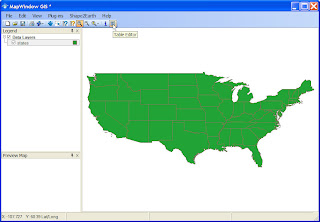 In order to normalize the data, we are going to use some of the tools that are already available in MapWindow. The first thing to do is open the table for states. This is done be selecting states in the table of contents, and then clicking the Table button (see above). This will open up the attribute table for the shapefile (below).
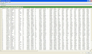
We are going to add a field to hold the normalized values. To do this, click Edit on the menu, and then select Add Field.
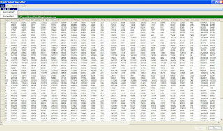 This will open up the Create Field dialog box (below). For this demonstration, we will create a field named "NormalizedMALES" that is of type "Double" (this will hold a numerical value for us).
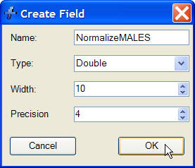
Once you hit OK, a new field will be added to the end of the table. Navigate to this field and right-click it. From the menu that appears, select Calculate Values (All Records).
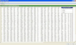 This selection will open up the Calculate Column Values dialog box. This is where we will enter the algorithm that creates the values in our normalized field.
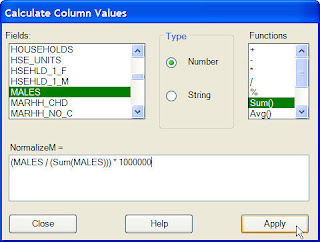
After you have entered the formula (above), click the Apply button. This will populate the new field you created with the normalized values.
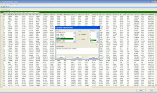
After hitting Apply, click Close to close the dialog box. Also make sure to click the Apply button at the bottom of the table before closing. This will save your newly created data.
Start off by loading the states.shp file (usually found at C:\_GE Data\Sample Projects\United States\Shapefiles\states.shp). MapWindow will assign a default color.
 In order to normalize the data, we are going to use some of the tools that are already available in MapWindow. The first thing to do is open the table for states. This is done be selecting states in the table of contents, and then clicking the Table button (see above). This will open up the attribute table for the shapefile (below).
We are going to add a field to hold the normalized values. To do this, click Edit on the menu, and then select Add Field.
 This will open up the Create Field dialog box (below). For this demonstration, we will create a field named "NormalizedMALES" that is of type "Double" (this will hold a numerical value for us).
Once you hit OK, a new field will be added to the end of the table. Navigate to this field and right-click it. From the menu that appears, select Calculate Values (All Records).
 This selection will open up the Calculate Column Values dialog box. This is where we will enter the algorithm that creates the values in our normalized field.
The algorithm entered below creates a ratio that is based off of the total population of males in from each state. The basic formula is (Males from State X) divided by (Total number of Males from all States). We then multiply the result by a factor that does nothing more than elevate the value so that the states will extrude far enough off of the surface to not intersect the Google Earth.
The formula used for this example is (MALES / (Sum(MALES))) * 1000000.
(NOTE: use of the multiplication factor is not really necessary if you do not plan to use this field as a height value. It also does not need to be nearly as big as the number we used here when using polygon features that are smaller than states, such as buildings.)

After you have entered the formula (above), click the Apply button. This will populate the new field you created with the normalized values.

After hitting Apply, click Close to close the dialog box. Also make sure to click the Apply button at the bottom of the table before closing. This will save your newly created data.
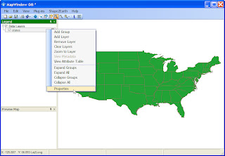
Now that we have a new field with normalized data, we will change the colors of each State based on this new value. Review the demonstration Changing Polygon Colors to see more information on changing colors. The two graphic below are a quick walk through of accessing the Properties and changing the colors.
One more step we will want to take is to spread out the color ramp. To do this, enter a number that is larger than the total number of records (in this case, 48 States).
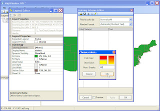 Red and Yellow have been selected as the ending and starting color, and 100 has been entered for the number of breaks. The spread values can be seen below.

Now we can see the normalize values in MapWindow. Notice how the color values have been much more spread out compared to the map created when we used the raw data in MALES field.
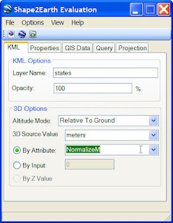 It is also a good idea to always select a Feature Name Field to name each of your Placemarks in Google Earth (see below).
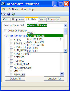
Finally, convert the data and load it into Google Earth. Compare this map to the one created with non-normalized data (viewable HERE).

One more step we will want to take is to spread out the color ramp. To do this, enter a number that is larger than the total number of records (in this case, 48 States).
 Red and Yellow have been selected as the ending and starting color, and 100 has been entered for the number of breaks. The spread values can be seen below.
Now we can see the normalize values in MapWindow. Notice how the color values have been much more spread out compared to the map created when we used the raw data in MALES field.
Now that we have our normalized data ready in MapWindow, we can convert it to KML for viewing in Google Earth.
Click Shape2Earth in the menu and select Export to KML. After Shape2Earth opens, change the Altitude Mode to Relative To Ground, click the By Attribute option, and then select the NormalizeMALE field from the drop down box (keep the 3D source value at Meters).
 It is also a good idea to always select a Feature Name Field to name each of your Placemarks in Google Earth (see below).
Finally, convert the data and load it into Google Earth. Compare this map to the one created with non-normalized data (viewable HERE).
This Google Earth map below is much easier to understand and easier to view.
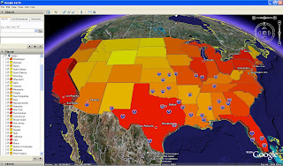 Normalized data is also very useful when not creating height values. The map below was created using the normalized data with the height set to Clamped to Earth, and the centerpoint label option selected.
 Normalized data is also very useful when not creating height values. The map below was created using the normalized data with the height set to Clamped to Earth, and the centerpoint label option selected.
Shape2Earth: Basic Polygon Height
Shape2Earth offers several options for creating 3D features from GIS data for viewing in Google Earth. This example uses the States shapefile used in the Basic Importing example, and sets unique values for each State shown in the Changing Polygon Colors example.
There are 4 basic options for dealing with height values in Google Earth. KML vector data can be clamped to the ground (all data lays directly on the ground with no height values used), data can be extruded relative to the ground (a height value of 5 meters will be extruded 5 meters above the ground at any given location), or height can have an absolute value (height is the actual height regardless of the underlying terrain; a point with a height of 5010 meters at a location with a height of 5000 meters will be 10 meters above the ground).
The fourth option for height uses the above options by applies to Collada models that can be loaded in Google Earth after Version 4. Models are not available in Shape2Earth 1.0, but may be made available later.
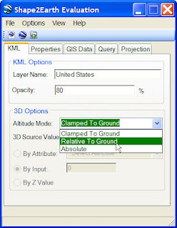 For this very simple example, we will select Relative To Ground as our height mode. When this is selected, the other 3D options in Shape2Earth are made available.
The first choice we will need to make is the unit to be used for height. The options given are Feet or Meters. For this example, we will select Feet.
(Note: All height units in KML are measured in meters. The Feet option in Shape2Earth converts to a metric equivalent for Google Earth)
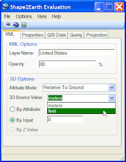 There are three different ways in Shape2Earth to get height values. You can use an attribute field in the GIS attribute data to use as a height, you can set a single arbitrary height that will be applied to all features, or you can use Z values in the GIS data itself (if they are present).
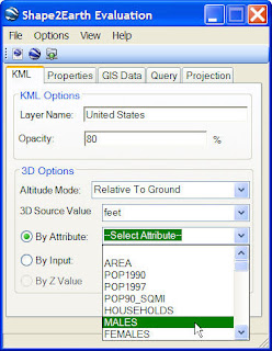
For this example, we are going to select an attribute field to use for height. The field selected was MALES (see below).
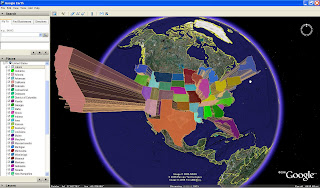
 Once we have set all selections for height, we can convert the data to KML and view it in Google Earth (below).
To make a more powerful map, we can associate the color of each State with the height. To do this, we will open the properties of the shapefile (right-click in the MapWindow table of contents and select 'Properties'), and then open the Coloring Scheme Editor (refer to Changing Polygon Colors for more information on changing colors)
There are 4 basic options for dealing with height values in Google Earth. KML vector data can be clamped to the ground (all data lays directly on the ground with no height values used), data can be extruded relative to the ground (a height value of 5 meters will be extruded 5 meters above the ground at any given location), or height can have an absolute value (height is the actual height regardless of the underlying terrain; a point with a height of 5010 meters at a location with a height of 5000 meters will be 10 meters above the ground).
The fourth option for height uses the above options by applies to Collada models that can be loaded in Google Earth after Version 4. Models are not available in Shape2Earth 1.0, but may be made available later.
 For this very simple example, we will select Relative To Ground as our height mode. When this is selected, the other 3D options in Shape2Earth are made available.
The first choice we will need to make is the unit to be used for height. The options given are Feet or Meters. For this example, we will select Feet.
(Note: All height units in KML are measured in meters. The Feet option in Shape2Earth converts to a metric equivalent for Google Earth)
 There are three different ways in Shape2Earth to get height values. You can use an attribute field in the GIS attribute data to use as a height, you can set a single arbitrary height that will be applied to all features, or you can use Z values in the GIS data itself (if they are present).
For this example, we are going to select an attribute field to use for height. The field selected was MALES (see below).
 Once we have set all selections for height, we can convert the data to KML and view it in Google Earth (below).
To make a more powerful map, we can associate the color of each State with the height. To do this, we will open the properties of the shapefile (right-click in the MapWindow table of contents and select 'Properties'), and then open the Coloring Scheme Editor (refer to Changing Polygon Colors for more information on changing colors)
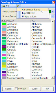
Once the Coloring Scheme Editor is open, select STATE_NAME as the Field to color by, and select Continuous Ramp (see below).
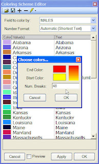
 Next, you will be given a form to select the beginning and ending color that will be used to color ramp between the high and low value. For this example, I have chosen Red for the end color (high value) and yellow for the start color (low value).
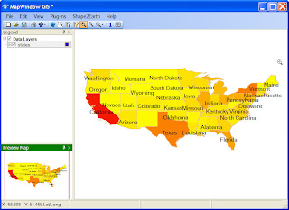
 The graphic below shows the color ramp applied to the data as seen in MapWindow.
And the graphic below shows this color scheme with the height values in Google Earth.
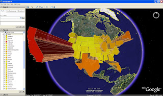
The graphic below is the same as above with the opacity level set to 100% (instead of 80% above).
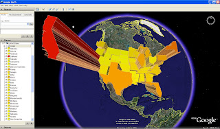
While this map does convey information pretty well, there are a couple of problems with it. For one, California is so high that it becomes difficult to see the other States. In situations like this, it might be a good idea to normalize your GIS data. Fortunately, there are a number of methods for normalizing data that can be done rather easily in MapWindow. (Refer to Normalizing GIS Data For Google Earth to learn how).
Return to Users Manual
 Next, you will be given a form to select the beginning and ending color that will be used to color ramp between the high and low value. For this example, I have chosen Red for the end color (high value) and yellow for the start color (low value).
 The graphic below shows the color ramp applied to the data as seen in MapWindow.
And the graphic below shows this color scheme with the height values in Google Earth.

The graphic below is the same as above with the opacity level set to 100% (instead of 80% above).

While this map does convey information pretty well, there are a couple of problems with it. For one, California is so high that it becomes difficult to see the other States. In situations like this, it might be a good idea to normalize your GIS data. Fortunately, there are a number of methods for normalizing data that can be done rather easily in MapWindow. (Refer to Normalizing GIS Data For Google Earth to learn how).
Return to Users Manual
Shape2Earth: Changing Polygon Colors
This section will show basic methods for changing the colors of polygons in MapWindow. The colors set in MapWindow are used by Shape2Earth when it renders the Keyhole Markup Language (KML) file for viewing GIS data in Google Earth. Basic information on loading data into MapWindow can be reviewed here.
We will start out with a basic shapefile loaded into MapWindow. When loaded MapWindow sets a default color for the shapefile. In the case below, the default was blue. If you are following along with MapWindow, your color might be different.
(Note: the shapefile used in this exercise is from the MapWindow installation, usually found at C:\Program Files\MapWindow\Sample Projects\United States\Shapefiles\states.shp).
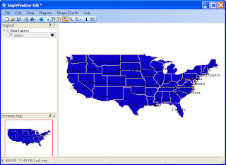
To change the color of the polygons, right-click on the shapefile name in the MapWindow table of contents and select Properties from the menu.
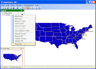
This will open up the MapWindow Legend Editor for the selected shapefile. The Legend Editor presents several options for changing the shapefile symbols. You can change both the Fill Color and the Line Color for the shapefile to get the color scheme you want. You can also set the colors of each individual feature based on a GIS attribute. This will allow you to create highly customizable GIS based maps for displaying in Google Earth.
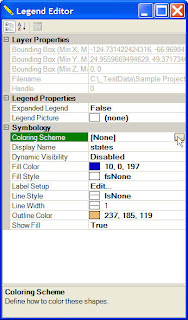 To set the color of each feature based on a GIS attribute, click on the Coloring Scheme value in the Legend Editor (see above). This will open up the Coloring Scheme Editor (below). The first thing you will need to do is to select the GIS attribute field whose values you would like to use for color coding. In this example, we are going to use the STATE_NAME field to uniquely color code each State.

Once you have selected the field you want to use, you will need to determine how you want to break up the data in that field to be color coded. MapWindow offers 3 options for cartagraphically organizing and displaying data using color.
You can use Continuous Ramp to make a smooth transition from one color to another based on attribute values. Any example of this method is shown HERE.
Equal Breaks allows users to organize data into specific color categories based on their attribute relationships.
Unique Values sets a color for each unique value. This is what we will use for this example.
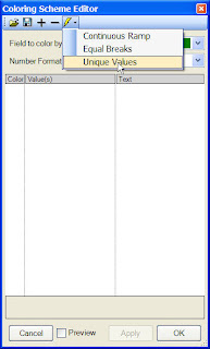
After you have selected Unique Value, the Coloring Scheme Editor will be populated by the unique values found in the selected attribute field, and will apply a random color to each unique value (see below).

Each individual color can me modified by the user simply by clicking on it. This will open the Color Editor which is used for selecting a cusomized color. In the example below, we are changing the color of the unique value 'Alabama' from Black to Green.
We will start out with a basic shapefile loaded into MapWindow. When loaded MapWindow sets a default color for the shapefile. In the case below, the default was blue. If you are following along with MapWindow, your color might be different.
(Note: the shapefile used in this exercise is from the MapWindow installation, usually found at C:\Program Files\MapWindow\Sample Projects\United States\Shapefiles\states.shp).

To change the color of the polygons, right-click on the shapefile name in the MapWindow table of contents and select Properties from the menu.

This will open up the MapWindow Legend Editor for the selected shapefile. The Legend Editor presents several options for changing the shapefile symbols. You can change both the Fill Color and the Line Color for the shapefile to get the color scheme you want. You can also set the colors of each individual feature based on a GIS attribute. This will allow you to create highly customizable GIS based maps for displaying in Google Earth.
 To set the color of each feature based on a GIS attribute, click on the Coloring Scheme value in the Legend Editor (see above). This will open up the Coloring Scheme Editor (below). The first thing you will need to do is to select the GIS attribute field whose values you would like to use for color coding. In this example, we are going to use the STATE_NAME field to uniquely color code each State.
Once you have selected the field you want to use, you will need to determine how you want to break up the data in that field to be color coded. MapWindow offers 3 options for cartagraphically organizing and displaying data using color.
You can use Continuous Ramp to make a smooth transition from one color to another based on attribute values. Any example of this method is shown HERE.
Equal Breaks allows users to organize data into specific color categories based on their attribute relationships.
Unique Values sets a color for each unique value. This is what we will use for this example.

After you have selected Unique Value, the Coloring Scheme Editor will be populated by the unique values found in the selected attribute field, and will apply a random color to each unique value (see below).

Each individual color can me modified by the user simply by clicking on it. This will open the Color Editor which is used for selecting a cusomized color. In the example below, we are changing the color of the unique value 'Alabama' from Black to Green.
Select a new color or define a custome one.
This process will change the colors of the data as seen in MapWindow below. These color schemes are what will be used by Shape2Earth to color code the KML data for viewing in Google Earth.
Subscribe to:
Comments (Atom)


